This article is an introduction to Sound Event Detection (SED). The article is aimed at anyone who wants to learn more about how to capture, use AI and machine learning to create insights in real time, based on incoming audio data in your own applications.
There is a broad variety of use cases both for the industry, for public spaces, in nature and created recreational areas as well as a range of indoor uses for healthcare, security, maintenance, home automation, consumer electronics etc – sounds are everywhere.
SED applications may include the sound of glassbreak, baby cry, toilet flush, gunshot detection and many other sounds that can be used for different types of security and safety solutions, in the home or in public areas. Predictive maintenance is a large application area where SED can be used to detect anomalies in machines or manufacturing processes.
While vision and how we recognize and analyse visual data, works by integrating visual stimuli into a whole picture or an entity; sounds could be regarded almost as the opposite, like a cluster of derivatives, comprised of all audible frequencies present at a given time segment somewhere, sitting there superimposed on top of each other.
We’ve probably always been interested in sounds ever since ears were developed, being able to recognize sounds and what they mean has probably saved our lives countless times over the years. Today there is also a plethora of ways to getting help by allowing computers to recognize sounds for us, and we’ll look into some of these methods and possibilities in more detail.
Before you can analyze sounds using machine learning or any other tool, you’ll have to catch them first. The process of capturing an analog sound, turning it into ones and zeros is called digitization, which is usually done by using an audio interface either separate or built-in to the motherboard or even on a single-chip computer.
Every time you sample sound, your recording sums up all the present differences in air pressure incoming in the form of waves at that precise moment. The more often you sample, the better the fidelity of the recording. As many of us can remember from physics class, you need to sample at twice the rate of the highest frequency you’re interested in studying later on in the computer. For example, the human ear can hear frequencies up to around 20kHz, so you’ll need to sample at a rate of at least 40kHz to be able to capture all the frequencies that we can hear. This theory, the Nyquist theorem, was brought about almost a hundred years ago by a fellow called Harry Nyquist, a Swedish-American pioneer in sound research born in 1889, who worked at Bell Labs and AT&T. Standard commercial sample rates are 48kHz and 44.1kHz e.g. for standard audio CDs.
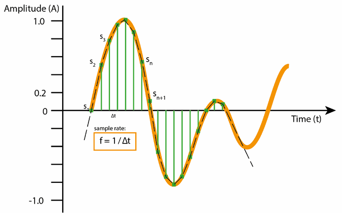
Each sound sample also has a depth to it, where consecutive discrete digital levels are chosen to mimic the true analog sine waves coming in. Letting 16 bits represent each sample, allows for 65,536 (216) possible values or 96dB range as your local Hi-Fi salesperson would like to put it. That’s already more than the range between the softest and loudest sound humans can hear. Audiophiles may argue that 24 or 32-bit representations (3 or 4 bytes per sample and channel) sound “better”, especially in the 2–5kHz range where we have our most range sensitivity, while for most applications two bytes per sample (16 bits) will do fine.
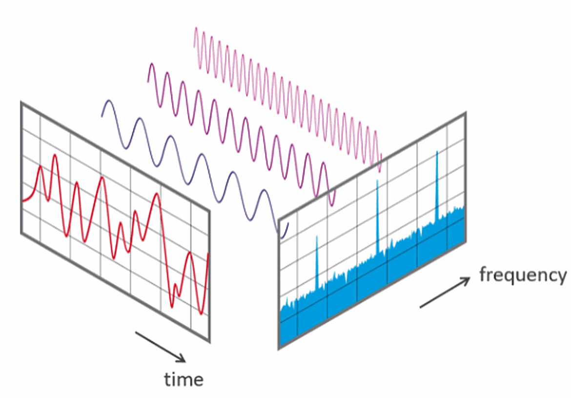
Once you have your piece of sound in the form of a succession of samples, you’ll be able to see the amplitude shift along the time axis. Looking at the curve plot won’t tell you that much about the frequencies involved and therefore the characteristics of the sound before you. By introducing one of mankind’s most useful functions; the Fourier transform, you’ll be able to collect information about what frequencies were used to build the sound wave, a bit like measuring what primary colors were used to make up a certain tint of mixed paint with one of those fancy pants spectrophotometers.
Unfortunately, as the Fourier transform works, you now lost the ability to pinpoint exactly when during your recorded sound’s duration that they occur. Yet, if your selected chunk was made up of say 400 samples, which at 40kHz sample rate represents 10 milliseconds worth of sound, you still have a good idea when a specific frequency occurs accurately enough for many practical applications. With time being the frequency inverted, this is long enough to depict a full 100 Hz or shorter sine waveform.
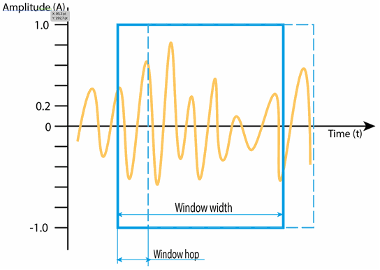
This short time chunk to be processed, is often called a Window in audio speak, for capturing a set of wavelengths of the recorded sound. Unfortunately, we seldom are lucky enough to neatly match with the exact start and end of one sine wave period, which in turn leads to some unwanted effects. In the frequency domain, we’ll typically see representations of very high frequencies which weren’t represented at all in the original sound but rather introduced in the process of rudely chopping off the ends when the Window of samples was selected.
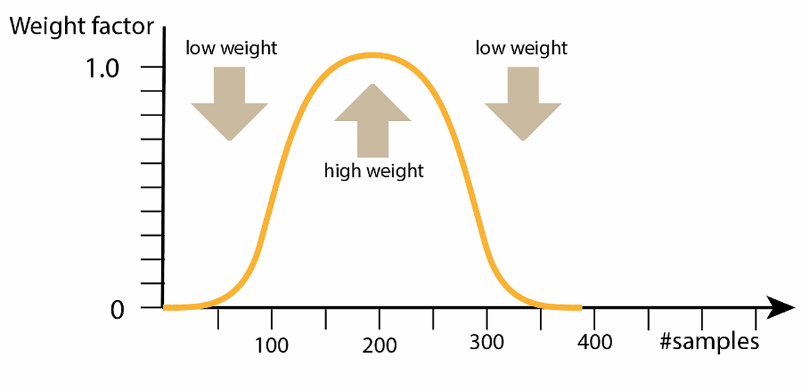
Luckily, there is a remedy for this by applying a weight function which emphasizes the middle section of the sound while suppressing pretty the end bits. One commonly used function is the Hamm window (ref Hamming-Hanning), looking much like a bell curve with multipliers near 1.0 in the middle, and near zero at the ends [figure X]. For noisy or unstable sounds, a function with a more narrow frequency response (e.g. Blackman) could be preferred of over Hamming-Hanning for tapering those end-points.
Friends of order may want to note that all parts of a window – also the ones near the chopped ends – need to be processed. To get all parts of a window accounted for, the final touch for solving this dilemma is to hop a shorter length along the timeline than one Window’s length, typically half a Window would do nicely to show this principle, so that we weigh in each part of the entire sound. In practice commercial software provides 8 times oversampling or more, resulting in smaller hops, better conservation of transients and more spectrogram strips with more similar representations.
By combining the amplitude and frequency plots gives you a spectrogram, which is a combined view with time on the x-axis, frequencies from the y-axis, and amplitudes from color. The louder the event the brighter the color, while silence is represented by dark color. It’s a convenient way to visually see patterns, and audio debris like noise and pauses.
As a result, we can extract a long train of overlapping windows with samples all of the same size suitable for training, feed into your favorite algorithm, and from which we can pull characteristics. Some features, like the dominating frequencies involved, the mean and max amplitude, and graphing the rise and decay of transients (amplitude envelope) don’t require the powers of machine learning and can easily be calculated from the data.
The sound recorded from a live environment is seldom well-formed for use directly though; there is always noise in the transducer (e.g. microphone, loudspeaker, or anywhere when energy is transformed from one form to another) and likewise background noise generated by unwanted sound sources. Sounds also occur at various loudness levels and at various timings, which need to be intelligently fitted in order to be comparable with the labeled data used in training. This calls for additional signal processing, with the purpose of extracting the relevant information from the data, and discarding the rest.
Some common signal processing techniques include:
Filtering
Filtering is the process of removing unwanted frequencies from a signal. This can be done using a low-pass filter to remove high frequencies, or a high-pass filter to remove low frequencies.
· Equalization
Equalization is the process of adjusting the level of different frequencies in a signal. This can be used to make a sound brighter or deeper, or to remove unwanted frequencies.
· Sound compression
Compression is the process of reducing the dynamic range of a signal. This can be used to make a sound louder, or also to reduce the level of background noise.
· Noise reduction
Noise reduction is the process of removing unwanted noise from a signal. This can be done using a noise gate, or by using a noise cancellation; mathematically subtracting a known ambient sound like in modern in-flight headphones popular in air travel.
· Reverberation
Reverberation is the process of adding artificial echo to a signal, and is more traditionally for human ears than machines. This is be used to make a sound more natural, or to make it match with sounds recorded in a room with different size or with surfaces where the sound could bounce.
From here, the choice of technique for the actual analysis is much up to the developer to find a tool appropriate for the application at hand; there are data models that require very little training to be useful, while others require the use of larger repositories of classified and labeled sounds to be successful.
One example of the latter is being able to identify and quantify the occurrences of bird song in the woods, for the purpose of doing inventory. Another kind of application, where the developer assumes that the sum of occurring noise levels from cars and other vehicles is proportional to the amount of pollution and effects on air quality. Here we don’t need to distinguish between car makes and models, just knowing that the sound originates from a car with a combustion engine will do nicely and hence less, and only more generic training data is required.
There is a plethora of ways to make computers recognize sounds, and we’ll look into some of them in more detail in upcoming articles. Here’s a brief overview:
1. Sonic tagging
Sonic tagging is where you give sounds unique identifier tags, much like QR codes, that can be read by a computer. This is useful for things like logging sounds made by machines in a factory, or for identifying birds by their songs.
2. Auditory scene analysis
Auditory scene analysis is the process of breaking down a soundscape into its component parts, so that the computer can recognize the individual sounds. This is useful for things like speech recognition, where the computer must be able to identify the different words that are being said.
3. Neural networks
Neural networks are a way of teaching computers to recognise patterns. They are often used for things like facial recognition, but they can also be used for sound recognition. Neural networks work particularly well with unstructured data (images, sound, signals) as they can learn non-linear mappings from input to the output prediction.
4. Deep learning
Deep learning is a subclass of machine learning that uses deep neural networks with many layers. Deep models can understand complex patterns in the data and are able to absorb and learn from large datasets. This is usually done by feeding the computer a training dataset, which has been labelled with the correct answers. The computer then tries to learn the patterns in the data, so that it can predict the correct labels for new data. Deep models have reached state-of-the-art performance in many different fields such as image recognition, audio classification and speech recognition.
5. Support vector machines
Support vector machines are a type of machine learning algorithm that can be used for sound recognition. They are often used for things like classifying images, but can also be used for sounds.
6. Template matching
Template matching is a way of recognizing sounds by comparing them to known templates. This is usually done by taking a recording of the sound, and then comparing it to a library of known sounds.
7. Hidden Markov models
Hidden Markov models are a type of statistical model that can be used for sound recognition. They are often used for speech recognition, but can also be used for other types of sound recognition.
8. Feature extraction
Feature extraction is the process of extracting interesting features from a sound. These features can then be used to train a machine learning algorithm.
9. Gaussian mixture models
Gaussian mixture models are a type of statistical model that can be used for sound recognition. They are similar to hidden Markov models but are more flexible and can be used for a wider range of sounds.
At Imagimob, we’re dedicated to help our customers to take tinyML SED applications to production by using deep learning techniques.
By forging partnerships with hardware companies, like AI chip makers Synaptics and Syntiant – we bring massive power to do advanced computing at the edge, allowing for local data processing and efficient sensor networking for many use-cases, for industry and societal needs allowing for better decision making in a broad range of uses.
Read more in upcoming articles in this series on tinyML for SED, and use cases on how customers use Imagimob AI to make applications fast and efficient!