
When building machine learning or artificial intelligence models, it’s easy to get started but sometimes your model performs badly and it is hard to understand why. In this guide, we will be looking at how to improve your models. While some of the tips will generalise to other types or areas of the field, our focus today will be on how to improve supervised learning models built for time-series data. Especially ones built for edge devices (tinyML), where inference or computation time (the time it takes for the embedded device to make one pass through the model) and memory footprint must be restricted to the devices capabilities.
There are two pathways to improving machine learning (ML) or artificial intelligence (AI) models. The first is data quantity and quality. This revolves around the data you have, how you got it and how much of it you got. The second is data processing, this involves getting a better understanding of your data and using that to help the model make the most out of the data you have. In this first section we will focus on the data quantity and quality. Looking into different things that need to be taken into account in order to maximise the performance.
You can find a breakdown at the end of the guide of everything covered. In this guide we will look at the following topics which we believe are great ways to make the most out of your model and data:
Data Quantity & Quality
Quantity and Quality of Data
Labelling
Class Weights
Data Processing
Understanding the Data
Processing the Data
Sliding Window
Advanced Pre-processor
Conclusion
There are a number of big points in this part, and the focus is on not only the quantity of data but the quality as well. Furthermore, how the data is labelled is also vital for ensuring good model performance.
It’s important to ensure that you have sufficient data. In general the more data the better. If one or more of your classes is performing badly you can try adding more data to see if that improves the situation or not. If things do not improve then you might have a data quality issue.
One indication of insufficient data is if you have a performance difference between your training and validation and between those and the test set.
When considering the data quality you need to think more deeply about what you’re trying to collect and how. Does your data contain all the relevant scenarios you're trying to identify? Does it accurately mimic a real world scenario? Are your sensors all configured correctly? When performing data collection it’s vital to ensure that all sensors used have:
You can intentionally set up systems with expected ranges of settings. For example, not every sensor needs to be oriented perfectly. This, however, needs to be factored in when you think about how much data you need. You need enough data of different types to ensure that the model is well accustomed to these deviations.
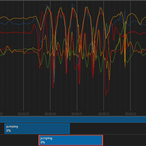
The next vital thing is the labelling, if there are labelling errors or there are some uncertain events that could cause a detrimental impact on the model. In the following figure, we can see that two labels are applied to the data. In the top one, the label starts a bit early and ends early whilst in the second one (highlighted in red), the label correctly encompasses the event. Poor labelling oftens leads to confusing the model, since it begins to learn that sometimes things other than jumps are also jumps and some things that are jumps are not to be classified as jumps. A few mislabelled data can ruin a batch of well labelled data. So it's always good to take a quick look at some of the data to see if that might be a possibility, especially in the classes that are performing badly.
As an extension since labels are applied over a period of time, the interaction between the window of data and the labels is done via the labelling strategy. Choosing the right labelling strategy for your project has a big impact. Label Strategy (Imagimob Specific) - using Imagimob AI you can select how your labels are applied to your sliding window, the strategy used can help change how the model behaves. Such is increasing model sensitivity or general performance. The important thing to think about in this case and when choosing the sliding window, is given a sliding window of the size that I have chosen, how does this apply to the data I have and how will they be labelled. When this window moves how will the labels change? This is especially crucial when you have classes of different times, or if the time of the event can differ drastically.
Another vital tool that can be used to influence the model performance is the class weights, which help influence the impact of that particular class on the loss function, giving it relatively more or less weight. Applying class weights can help to minimise the impacts of unbalanced classes. Unbalanced classes are those where one of the classes that you’re trying to identify might have significantly more or less data than the rest. In the following figure we can see for example that the push data is half the other two classes. We have 2 options, collect more push data or increase the class weight to 2.
As a starting point, balancing out the different classes proportionally is good. This can also be tweaked to improve the performance, either raising it to make a class more prominent or reducing it to make a class less prominent.
Previously we talked about the data quantity and quality and how to maximise the potential in those, once you have reached a good point in those the next step is to look at the data processing. But, before you process the data you must first understand it. What we mean by this; is thinking about the sensors used in the particular application, how the sensors generate their data and how the data is expected to behave under the conditions of what is to be classified. Understanding your data is vital to ensuring you have sufficient model performance. Once you understand it then you can process it. Processing it is significant to improving model performance.
For example, say you have a fall detection algorithm, one that uses an accelerometer. You know that you’ll have the following states:
This is a simple example but it shows the steps taken to take a complicated task and breaking it down to try to understand the sensor (accelerometer) behaviour during different parts of the event we want to classify (fall). The processing then focuses on how to highlight certain parts of the data to make it easier or clearer for the model. Things like extracting the magnitude helps to identify the 1g point, low pass filters help to track the free-fall, whereas high pass filters help make the impact more prominent.
The best way to get an understanding of the data is to visualise it. Typically this is a simple plot of the data signals. One step further is to visualise the data and to compare it to a video with the real event. This allows you to correlate the data traits and features with what’s happening in a real life scenario. Following the aforementioned example of free-fall, it’s very basic, but you’ll quickly learn that if a sensor is placed on a human the human will not simply fall flat but the human will move to protect themselves during a fall. These movements are typically dominant. It makes sense when you compare the video with the data but when just looking at the data it is not so clear. This is a simple example, in more extreme cases this becomes even more crucial.
Furthermore, sometimes the raw data from the sensor is not the best for humans or the ML model to understand. This is where data processing or pre-processing becomes important!
As mentioned previously, sometimes to squeeze out more values from the data you need to process it. This could be anything from scaling or normalising it, to transforming it to the frequency domain or even just simplify filtering it to remove noise. There’s also the fact that typically time-series data is fed using a sliding window so that you add the time aspect as well. First we will explain the sliding window and how to get the information out then we will go to the more advanced processing tools later.
In state-less models, time-series data is typically fed as a window. This allows the model to get information about the data over a period of time. When configuring your sliding window there are two parameters to fine tune. Those are:
Now, the main thing here is that we are assuming a synchronous system where the data sampling occurs at a constant rate. In the span of this document we will not go into asynchronous systems with non-constant sampling rate. Furthermore, this is more relevant for state-less models as opposed to state-ful where you don’t typically have a sliding window.
The Window Length is the size of the window, how many samples of data you will have, and by extension the length of time that you will observe at any one time. It’s generally easier to think about the window length in terms of time, you may want your window to be 2 seconds for example. To convert between the two units is very simple and you can think of it by the following equation:
Window Length =t(window) × f(sampling)
This means that you simply multiply the desired time length by the sampling frequency to obtain the length of your window. This is your starting point, you typically want to see how your model reacts to slightly different window lengths, especially if you have classes of different sizes. For example if you are running, your individual steps will happen quickly but if in the same model you want to classify jumping then you want a bigger window. You may then resort to having a window that is more tuned to the slower event.
Next is the stride, the stride is less vital to the performance but it is something to be wary of. You could have a stride of 1 and this would result in good performance. This, however, is very resource intensive, in terms of model training this would result in lengthy iterations and in terms of model deployment such models usually lead to problems where the compute time required is longer than the sampling period. But, on the other hand, having a stride value that’s too high means that your window might entirely bypass the event. Given this information, a general approach is to start with a stride value of half the sampling window then begin fine tuning for performance vs. compute time trade off.
Finally, we reach the pre-processing. Pre-processing refers to all the processing applied before the data is passed to the neutral network. In this case we consider anything beyond a simple sliding window as advanced pre-processing. At this point, you are free to draw on centuries of research into different topics. At this point is where you can utilise in studies you’ve done in the subject or dig into other’s research into the topic. There are endless possibilities in terms of the pre-processing but we will touch on some common ones in hopes of giving inspiration for you to build on top of it and implement your own.
Filtering is very common for time-series data. You can filter to hide unwanted data so that the model has an easier time of identifying the correct events or you can filter to highlight important information in the data. The are 4 types of filters:
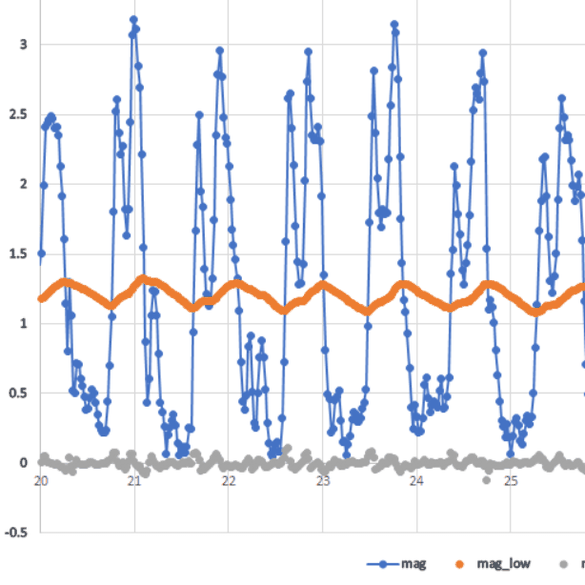
One particular example is human motion, if a sensor is placed on the back then you expect that the person cannot move very quickly so you can use the high frequency components to disqualify or highlight false positives. The following figure shows an accelerometer magnitude of a person jumping. We see the raw signal, a low pass filtered and a high pass filtered signal.
Another powerful tool is a fourier transform. What this does is that it transforms the time-domain data into its frequency components in the frequency domain.
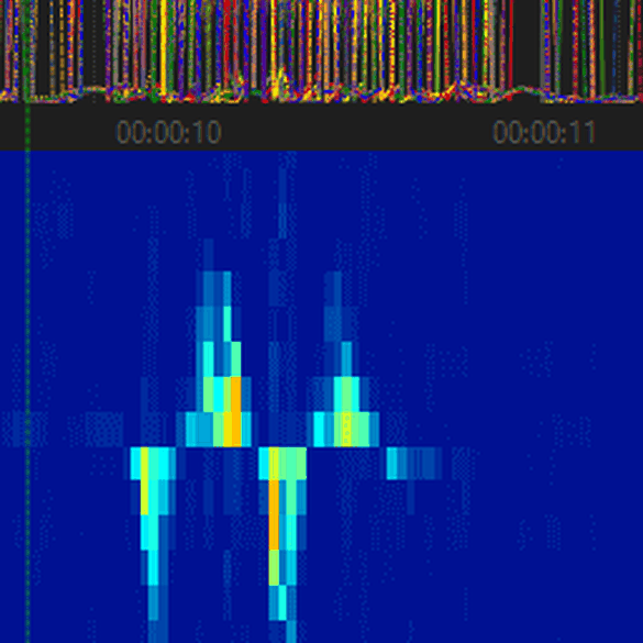
This sometimes shows more information and highlights different properties of the data. In the following example you see the effects of transforming many signals into a heat spectrum by performing a fourier transform. What was previously unintelligible or hard to decipher becomes very clear and something that could help to build a compact and great performing model.
There are a lot of important factors that go into getting the most out of your machine learning model. Previously we looked at the following points:
If you’re having trouble with your model, take a step back and think about all these components. Try adjusting one of the variables in your system and train a couple of different models with bigger or smaller values and see its impact. For example try slightly bigger and slightly smaller than your current sliding window size, which performed better? What if you change it further in that direction? Is it better or worse?
These are the questions that you should ask yourself as you are building your models. Tamper, tweak and experiment.